Energy Forecast for a full-scale Vehicle Plant
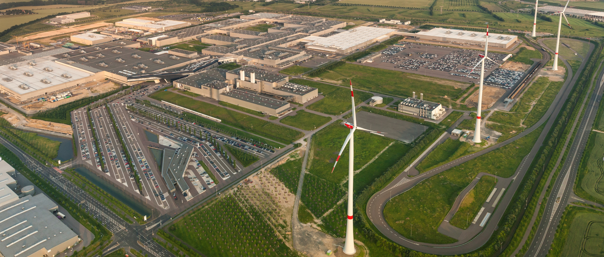
Energy Forecast for a full scale Vehicle Plant
Energy forecasting is based on time series analysis. There are many techniques for analysing and forecasting time series, e.g. ARIMA, linear regression and deep learning. To tackle the challenge at hand a linear regression will be the benchmark model aganst which deep learning models will be tested. In particular a multi layer perceptron (MLP) and recurrent neural network (RNN), i.e. Long-Short Time Memory (LSTM) model will be applied.
Business Domain
Energy forecasting is a tricky challenge because many factors might influence the final energy demand of a complex system like a large manufacturing plant. Especially when the plant employs not only energy consumers but also energy producers like CHPs and wind farms or energy reservoirs like battery farms. Significant factors to take into account:
- production plan
- CHP energy production
- weather, i.e. temperature, wind
Data Preparation
In order to apply the described techniques the problem has to be framed as a supervised learning problem. The data at hand is an hourly measurment of energy consumption in 2015 as well as associated production plans and weather data. This results to a multivariate time series. The variable to forecast is energy consumption for the next 48 hours.
For application in a LSTM neural network with tanh non-linearity the data need to be scaled to the interval [-1,1]. Furthermore we split it into a training set (80%) and a test set (20%).
For forecasting different tactics can be applied.
- Linear regression: the timesteps are taken as independent from the past an only dependent on the feature vector at time t=0.
- MLP: similar to linear regression with respect to feature preparation.
- LSTM: the timesteps are dependent on their predecessors and therefor the see-behind window is a hyperparameter to be chosen for the model.
For this analysis the LSTM model will have two variants with regards to the lookback window:
- the entire dataset will be taken as sequence length, i.e. the LSTM context will be build over the entire time series. In Keras this results in a statfull LSTM network with batch-size 1 (online learning)..
- a lookback window of 14days will be taken. This allows for batch-size > 0 and a stateless LSTM network.
For the non RNN models also information from previous timesteps can be encoded into the feature vector by just putting the values of past timesteps as additional features into the feature vector. Here we also use the information of the last 14 days to be consistent within our model choices.
For all models the following parameters/features have been selected:
- energy consumption
- air temperature
- wind speed
- wind direction
- production plan
This results in a feature vector for the linear models of dimension 1872:
- lookback: 14days24h5features
- lookforward: 2days24h4features (5th parameter is the energy and is the label in our models to be forecasted)
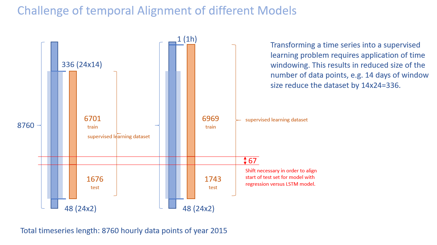
Timestamp Challenges
Keeping the timestamps correct after all the data transformations is a special challenge which requires careful handling. The following diagram illustrates the topic. Left you can see the resulting dataset for a lookback window of 14days whereas on the right for a lookback window of 1hour. In order to compare results, the inverse date transformations have to take this into account.
Model
We predict the entire 48 hours with one prediction in order to avoid instabilities introduced by step-by-step forecasting and then using the forecast as feature for the next forecast.
For the linear regression the venerable scikit-learn library is used. For all the deep-learning KERAS and TENSORFLOW are the tools of choice.
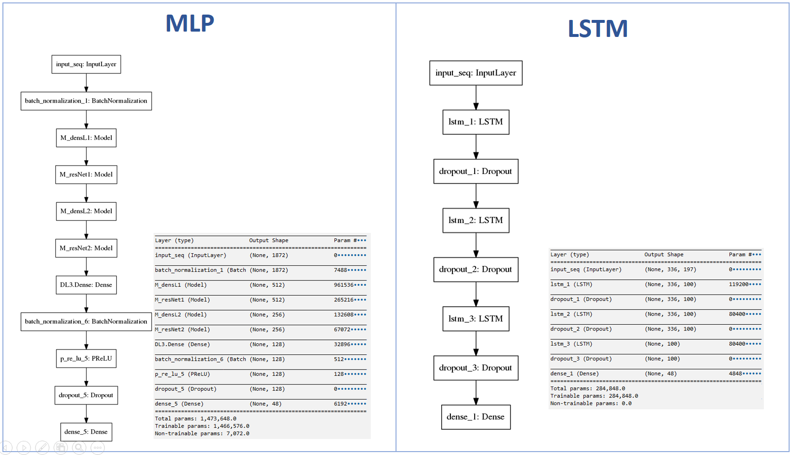
The MLP model has got 1.4 Mio parameters, so its capacity is much higher then the LSTM. This gives already a first hint towards further optimization of model setup.
Result
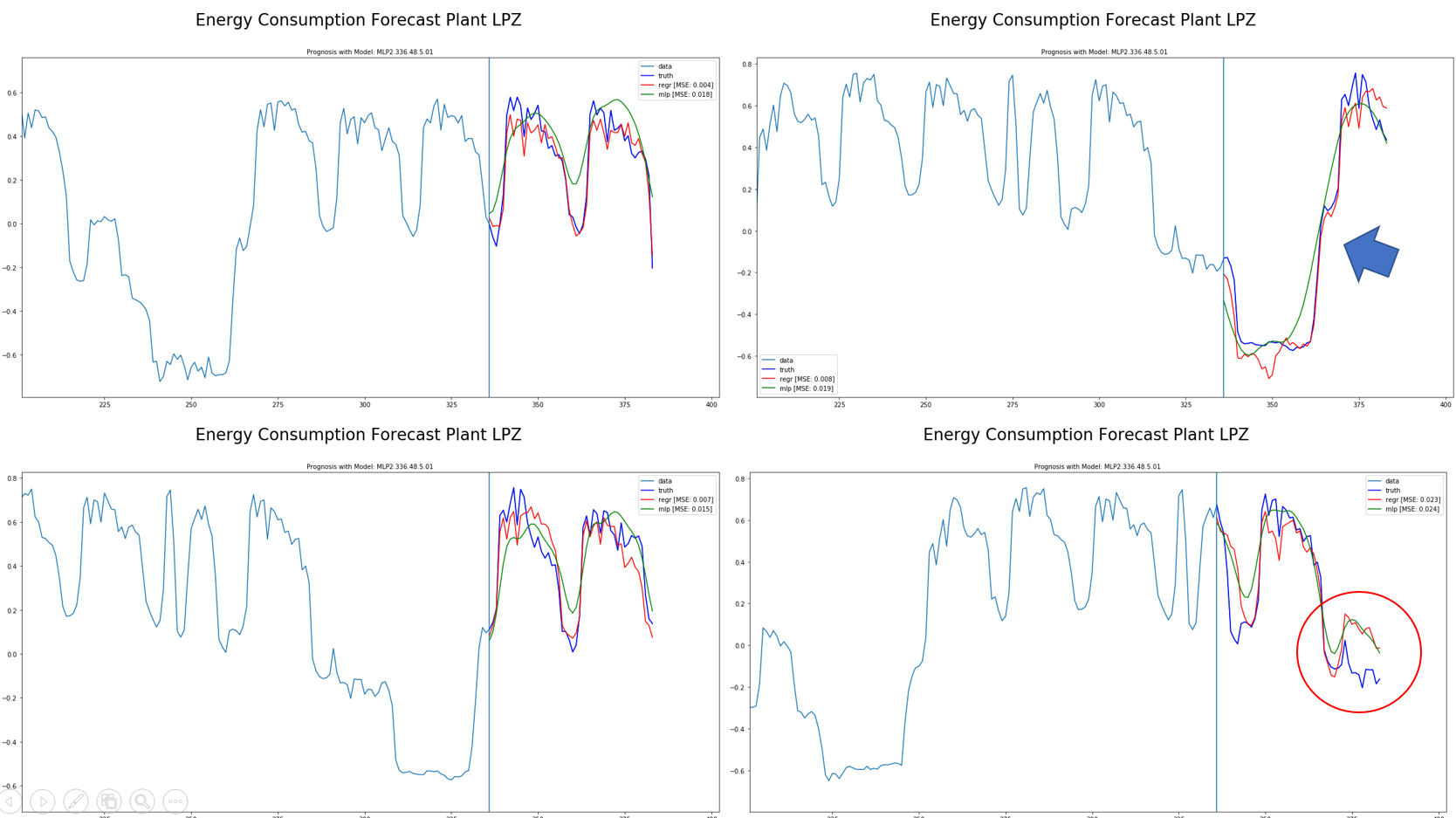
Quality of forecast is measured as MSE (mean squared error). All plots show an arbitrary point in time of the test set with 14days in the past and 2 days forecast. Every model is compared to the naive linear regression (red line).
LTSM
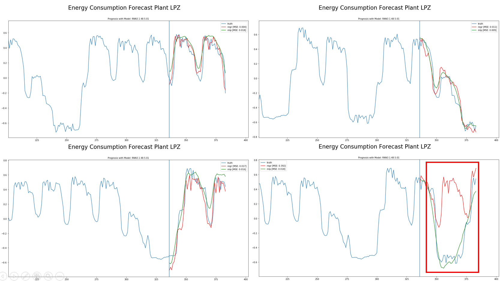
The LTSM model overall shows an MSE of 0.025 on the test set.
The red box shows an outlier in the linear regression. It seems like the linear model did not pick up a significant feature like production plan properly. The LSTM did a better job here.
MLP
The MLP model overall shows an MSE of 0.063 on the test set.
Conclusion
Although both deep learning approaches can predict the shape of the time series well, the LSTM model exhibits higher accuracy. Since the model capacity is much lower, this was a surprising outcome.
However both deep learning approaches seem struggle to match the quality of a simple linear regression forecast. Due to time contraints no hyperparameter or model tuning has taken place. There are many areas for potential improvements, e.g.
- detailed feature preparation, especially production plans
- exploration of more neural network configurations (number of layers, number of timesteps, number of neurons, …)
- hyperparameter tuning (regularization, learning rates, optimiziers, …)
Thanks for reading.