Cheat Sheet

General Explanations:

• embeddings: a way to translate multidimensional input into fixed length log dimensional representations: lookup the integer index of the object and look it up in a corresponding matrix wich holds the low-dim representation. If no embeddings are used, the input has to be one-hot-encoded wich yields huge matrices
• KFold Cross Validation: The purpose of cross-validation is model checking, not model building. Once we have used cross-validation to select the better performing model, we train that model (whether it be the linear regression or the neural network) on all the data. We don’t use the actual model instances we trained during cross-validation for our final predictive model.
• A dense layer in a multilayer perceptron (MLP) is a lot more feature intensive than a convolutional layer. People use convolutional nets with subsampling precisely because they get to aggressively prune the features they’re computing.
• in NNs rarely occur local minima due to vast parameter space (probability not to get better in ayn dimension is miniscule)
• the fast majority of space of a loss function in NN is all saddlepoints
• one training cycle for the entire dataset is called epoch, i.e. the algorithm sees the ENTIRE dataset
• iteration: every time a batch is passed through the NN (forward + backward pass)
• Latent factors = features of embeddings (used in Collaborative Filtering)
• Bias-Variance Tradeoff in Machine Learning
• Softmax vs Sigmoid: All the softmax units in a layer are constrained to add up to 1, whereas sigmoid units don’t have this ’lateral’ constraint. If every example can be associated with multiple labels, you need to use a sigmoid output layer that learns to predict “yes” or “no” for each individual label. If the classes are disjoint, i.e. each example can only belong to one class, you should use a softmax output layer to incorporate this constraint.
• Do not forget to fine tune your network architecture and your learning rate. If you have more data, a complex network is preferable. According to one important deep learning theorem, the local minima are very close to the global minimum for very deep neural networks.

Preprocessing

• pre-process your data by making sure each dimension has 0 mean and unit variance. This should always be the case with data your are feeding to a NN, unless you have strong, well-understood reasons not to do it. A simple MLP will never cause gradient explosion if your data is correctly preprocessed.
• Centering sparse data would destroy the sparseness structure in the data, and thus rarely is a sensible thing to do.
• However, it can make sense to scale sparse inputs, especially if features are on different scales.
• MaxAbsScaler and maxabs_scale were specifically designed for scaling sparse data, and are the recommended way to go

Underfitting/Overfitting

• Underfitting: This describes a model that lacks the complexity to accurately capture the complexity inherent in the problem you’re trying to solve. We can recognize this when our training error is much lower than our validation error
• Overfitting: This describes a model that is using too many parameters and has been trained too long. Specifically, it has learned how to match your exact training images to classes, but has become so specific that it is unable to generalize to similar images. This is easily recognizable when your training set accuracy is much higher than your validation.
• when you start overfitting you know, that your model is complex enough to handle your data
• Your main focus for fighting overfitting should be the entropic capacity of your model –how much information your model is allowed to store. A model that can store a lot of information has the potential to be more accurate by leveraging more features, but it is also more at risk to start storing irrelevant features. Meanwhile, a model that can only store a few features will have to focus on the most significant features found in the data, and these are more likely to be truly relevant and to generalize better.
• Dropout also helps reduce overfitting, by preventing a layer from seeing twice the exact same pattern, thus acting in a way analoguous to data augmentation (you could say that both dropout and data augmentation tend to disrupt random correlations occuring in your data).

Recipe:

1. Add more data
2. Use data augmentation
3. Use architectures that generalize well
4. Add regularization
5. Reduce architecture complexity.

Recommendation and Tricks

General

• be aware of the curse of dimensionality
• less parameter tend to generalize better
• there is no inherent problem with using an SVM (or other regularised model such as ridge regression, LARS, Lasso, elastic net etc.) on a problem with only 120 observations but thousands of attributes, provided the regularisation parameters are tuned properly.
• Rule of thumb: number of parameters > number of examples = trouble
• different input/pic sizes: final Dense layer does not work, all others don’t care of the input size, so to create the conv-features, you can use any size
• make the first Keras layer a batchNorm layer, it does normalization for you and allows for higher learning rates
• regularization you cannot do on a sample, to understand how much regularization is necessary you need the entire dataset
• for kaggle use clipping to avoid the logloss problem!!!
• convnet: any kind of data with consistent ordering, audio, consistent timeseries, ordered data
• instead of one-hot-encoding the labels(target) we can use a cool optimizer in keras: loss='sparse_categorical_crossentropy' takes an integer target (categorical_crossentropy takes one-hot-encoded target)
• When the dataset size is limited, it seems augmenting the training labels is just as important as augmenting the training data (i.e. image perturbation)
• if you deep net is not working, then use less hidden layers, until it works (simplify)

General Neural Networks

• Unless you want to know which are the informative attributes, it is usually better to skip feature selection step and just use regularization to avoid over-fitting the data.
• We no longer need to extract features when using deep learning methods as we are performing automatic feature learning. A great benefit of the approach.
• functional model in keras allows adding metadata on later layers, e.g. image size after the conv-layers so that dense layers have this information to work with

Dropout

• Today dropout starts in early layers with .1/.2 … .5 for the connected layers
• Dropout eliminates information just like random forests (randomly selected new models)

Data Augmentation

• no augmentation for validation sets
• vertical flippings? do you see cats on their head?
• use channel augmentation

Pseudo Labeling, Semi-Supervised Learning

• One remarkably simple approach to utilizing unlabelled data is known as psuedo-labeling. Suppose we have a model that has been trained on labelled data, and the model produces reasonably well validation metrics. We can simply use this model then to make predictions on all of our unlabelled data, and then use those predictions as labels themselves. This works because while we know that our predictions are not the true labels, we have reason to suspect that they are fairly accurate. Thus, if we now train on our labelled and psuedo-labeled data we can build a more powerful model by utilizing the information in the previously unlabelled data to better learn the general structure.
• One parameter to be mindful of in psuedo-labeling is the proportion of true labels and psuedo-labels in each batch. We want our psuedo-labels to enhance our understanding of the general structure by extending our existing knowledge of it. If we allow our batches to consist entirely of psuedo-labeled inputs, then our batch is no longer a valid representation of the true structure. The general rule of thumb is to have 1/4-1/3 of your batches be psuedo-labeled.
• Pseudo-Labeling: ca. 30% in a batch

Training

• online learning (batch size=1): network update foreach training example -> quick, but can be chaotic
• batch learning: save the errors across all training examples and update network at the end -> more stable, typical batch size 10-100
• larger batch is always better. The rule of thumbs is to have the largest possible batch your GPU can handle. The bigger your gradients are, the more accurate and smooth they will be. If you have batch_size=1, you can still converge to an optimal value, but it will be way more chaotic (much higher variance but still unbiased). And it will be way slower!
• If network doesn’t fit, decrease the batch size, since most of the memory is usually consumed by the activations.
• start with a very small learning rate until the loss function is better then baseline chance
• Batchnorm: 10x or more improvements in training speed. Because normalization greatly reduces the ability of a small number of outlying inputs to over-influence the training, it also tends to reduce overfitting.
• Having Batch Norm added, can allow us to increase the Learning Rate, since BN will allow our activations to make sure it doesn’t go really high or really low.
• use RMSprop, much faster than SGD
• to continue training: just call .fit one or several times and you will be able to continue to train the model. If you want to continue the training in another process, you just have to load the weights and call model.fit()
• fchollet: compiling a model does not modify its state. Weights after compilation are the same as before compilation.
• keras: compiling the model does does not hurt, however, changing trainable=true does not require it since the model does not change, only the metadata
• Sanity check: Overfit a tiny subset of data. try to train on a tiny portion (e.g. 20 examples) of your data and make sure you can achieve zero cost. Set regularization to zero, otherwise this can prevent from getting zero cost. Unless you pass this sanity check with a small dataset it is not worth proceeding to the full dataset. Note that it may happen that you can overfit very small dataset but still have an incorrect implementation. For instance, if your datapoints’ features are random due to some bug, then it will be possible to overfit your small training set but you will never notice any generalization when you fold it your full dataset ([source]http://cs231n.github.io/neural-networks-3/#gradcheck)
• increasing the regularization strength should increase the los
• Look for correct loss at chance performance (Regularization strength zero). For example, for CIFAR-10 with a Softmax classifier initial loss should be 2.302, because we expect a diffuse probability of 0.1 for each class (since there are 10 classes), and Softmax loss is the negative log probability of the correct class so: -ln(0.1) = 2.302.
• Validation accuracy can remain flat while the loss gets worse as long as the scores don’t cross the threshold where the predicted class changes.
• Don’t let the regularization overwhelm the data. Loss function is a sum of the data loss and the regularization loss (e.g. L2 penalty on weights). Regularization loss may overwhelm the data loss, in which case the gradients will be primarily coming from the regularization term (which usually has a much simpler gradient expression).
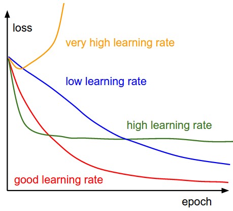
• Traing curves:

  

Transfer Learning

• Fully connected network localizes the interesting part in transfer learning to your specific problem domain
• start with the weights at the trained level, don’t randomize!

Data Leakage/Metadata

• often the main data already encorporates the added metadata, so it does not improve (e.g. pic size of fisherboats in fishing competition: 8 boats the net already learned about from the pics)
• metadata often is not worth the effort

Batchnorm, Batch Normalization

• It normalizes each layer
• can be used to just normalize data at the input layer.
• There are some additional steps that Batch Norm offers to make it work with SGD(the activations):
  • Adds 2 more trainable parameters to each layer.
    • One for multiplying the activations and set an arbitrary Standard Deviation.
    • The other for adding all the activations and set an arbitrary Mean.
    • BN (Batch Norm) doesn’t change all the weights, but only those two parameters with the activations. This makes it more stable in practice.

Hyperparameters:

• Hyperparameter ranges. Search for hyperparameters on log scale. learning_rate = 10 ** uniform(-6, 1). The same strategy should be used for the regularization strength. This is because learning rate and regularization strength have multiplicative effects on the training dynamics.
• Prefer random search to grid search.

Architecture

Rule of thumb: For a three layer network with n input and m output neurons, the hidden layer would have sqrt(n*m) neurons.

number of hidden layers

• 0 - Only capable of representing linear separable functions or decisions.
• 1 - Can approximate any function that contains a continuous mapping from one finite space to another.
• 2 - Can represent an arbitrary decision boundary to arbitrary accuracy with rational activation functions and can approximate any smooth mapping to any accuracy.

Ensembles

• Train multiple independent models, and at test time average their predictions. As the number of models in the ensemble increases, the performance typically monotonically improves (though with diminishing returns). The improvements are more dramatic with higher model variety in the ensemble.

CNNs

• network will not learn duplicate filters because this is not OPTIMAL
• A typical 2D convolution applied to an RGB image would have a filter shape of (3, filter_height, filter_width), so it combines information from all channels into a 2D output.
• If you wanted to process each color separately (and equally), you would use a 3D convolution with filter shape (1, filter_height, filter_width).
• conv-layers are compute intensive, dense layers are memory intensive
• 1D convolution is useful for data with local structure in one dimension, like audio or other time series.
• Note that sometimes the parameter sharing assumption may not make sense. This is especially the case when the input images to a ConvNet have some specific centered structure, where we should expect, for example, that completely different features should be learned on one side of the image than another. One practical example is when the input are faces that have been centered in the image. You might expect that different eye-specific or hair-specific features could (and should) be learned in different spatial locations.
• In that case it is common to relax the parameter sharing scheme, and instead simply call the layer a Locally-Connected Layer.

Systematic analysis of CNN parameters:

https://arxiv.org/pdf/1606.02228.pdf

• use ELU non-linearity without batchnorm or ReLU with it.
• apply a learned colorspace transformation of RGB.
• use the linear learning rate decay policy.
• use a sum of the average and max pooling layers.
• use mini-batch size around 128 or 256. If this is too big for your GPU, decrease the learning rate proportionally to the batch size.
• use fully-connected layers as convolutional and average the predictions for the final decision.
• when investing in increasing training set size, check if a plateau has not been reach.
• cleanliness of the data is more important then the size.
• if you cannot increase the input image size, reduce the stride in the consequent layers, it has roughly the same effect.
• if your network has a complex and highly optimized architecture, like e.g. GoogLeNet, be careful with modifications.
• maxpooling helps with translation invariance, helps find larger features, helpfull for any kind of convnets
• maxpooling: you only care about the most ‘dogginess’ of the picture, not the rest - better for pics where target is only small part of pic
• averagepooling: you care about more of the entire picture not only the extremes - better for pics with one filling motive
• Resnet has good regularization characteristics, authors do not include Dropout

RNNs

Predict multiple steps

1. “Function to Function Regression” which assumes that at the end of RNN, we are going to predict a curve. So use a multilayer perceptron at the end of RNN to predict multiple steps ahead. Suppose you have a time series and you want to use its samples from 1, …, t to predict the ones in t+1, …, T. You use an RNN to learn a D dimensional representation for the first part of time series and then use a (D x (T-t)) MLP to forecast the second half of the time series. In practice, you do these two steps in a supervised way; i.e., you learn representations that improve the quality of the forecast.
2. tbd

LSTM

The first dimension in Keras is the batch dimension. It can be any size, as long as it is the same for inputs and targets. When dealing with LSTMs, the batch dimension is the number of sequences, not the length of the sequence.

• LSTMs in Keras are typically used on 3d data (batch dimension, timesteps, features).
• LSTM without return_sequences will output (batch dimension, output features)
• LSTM with return_sequences will output (batch dimension, timesteps, output features)

Basic timeseries data has an input shape (number of sequences, steps, features). Target is (number of sequences, steps, targets). Use an LSTM with return_sequences.

stackoverflow

One-to-one: equivalent to MLP.

model.add(Dense(output_size, input_shape=input_shape))

One-to-many: this option is not supported well, but this is a workaround:

model.add(RepeatVector(number_of_times, input_shape=input_shape))
model.add(LSTM(output_size, return_sequences=True))

Many-to-one::

model = Sequential()
model.add(LSTM(n, input_shape=(timesteps, data_dim)))

Many-to-many: This is the easiest snippet when length of input and output matches the number of reccurent steps:

model = Sequential()
model.add(LSTM(n, input_shape=(timesteps, data_dim), return_sequences=True))

Many-to-many when number of steps differ from input/output length: this is hard in Keras. I did not find any code snippets to code that.

Tricks

• Within a batch, each sequence has its OWN states. Also each sequence is seen as independent from the other sequences in the batch. If your batch is Y, sequences Y[1] and Y[2] will never have something in common (whatever stateful=False or stateful=True).
• If the LSTM has the stateful mode, the states of the current batch will be propagated to the next batch (at index i). Batching sequences is only to speed up the computations on a GPU.
• 3 weight matrices: input, recurring, output
• fchollet: seq_len 100 seems large fora LSTM, Try 32
• if there is one step lag between the actual time series, this is the most seen “trap” if you do time series prediction, in which the NN will always mimic previous input of time series. The function learned is only an one-step lag identity (mimic) prediction (trivial identity function).
• The back propagation horizon is limited to the second dimension of the input sequence. i.e. if your data is of type (num_sequences, num_time_steps_per_seq, data_dim) then back prop is done over a time horizon of value num_time_steps_per_seq (https://github.com/fchollet/keras/issues/3669)
• all a stateful RNN does is remember the last activation. So if you have a large input sequence and break it up in smaller sequences, the activation in the network is retained in the network after processing the first sequence and therefore affects the activations in the network when processing the second sequence.
• Keep all long term memory when modelling Time Series where you may have very long term memory and when you don’t know exactly when to cut. No subsampling here.
• Recursive prediction of timesteps (multi-step) eventually uses values already predicted. This produces an accumulation of errors, which may grow very fast.

Optimiziers

• better than adagrad: rmsprop, it does not explode, just jump around, when it flattens out you should device learning rate by 10-100
• momentum + rmsprop = good idea -> adam
• SGD is well understood and a great place to start. ADAM is fast and gives good results and I often use it in practice.
• illustration (Images credit: Alec Radford):

  

  

Momentum (0.9)

For NN’s,the hypersurface defined by our loss function often includes saddle points. These are areas where the gradient of the loss function often becomes very small in one or more axes, but there is no minima present. When the gradient is very small, this necessarily slows the gradient descent process down; this is of course what we desire when approaching a minima, but is detrimental otherwise. Momentum is intended to help speed the optimisation process through cases like this, to avoid getting stuck in these “shallow valleys”.

Momentum works by adding a new term to the update function, in addition to the gradient term. The added term can be thought of as the average of the previous gradients. Thus if the previous gradients were zig zagging through a saddle point, their average will be along the valley of the saddle point. Therefore, when we update our weights, we first move opposite the gradient. Then, we also move in the direction of the average of our last few gradients. This allows us to mitigate zig-zagging through valleys by forcing us along the average direction we’re zig-zagging towards.

Adagrad

Adagrad is a technique that adjusts the learning rate for each individual parameter, based on the previous gradients for that parameter. Essentially, the idea is that if previous gradients were large, the new learning rate will be small, and vice versa.

The implementation looks at the gradients that were previously calculated for a parameter, then squares all of these gradients (which ignores the sign and only considers the magnitude), adds all of the squares together, and then takes the square root (otherwise known as the l2-norm). For the next epoch, the learning rate for this parameter is the overall learning rate divided by the l2-norm of prior updates. Therefore, if the l2-norm is large, the learning rate will be small; if it is small, the learning rate will be large.

Conceptually, this is a good idea. We know that typically, we want to our step sizes to be small when approaching minima. When they’re too large, we run the risk of bouncing out of minima. However there is no way for us to easily tell when we’re in a possible minima or not, so it’s difficult to recognize this situation and adjust accordingly. Adagrad attempts to do this by operating under the assumption that the larger the distance a parameter has traveled through optimization, the more likely it is to be near a minima; therefore, as the parameter covers larger distances, let’s decrease that parameter’s learning rate to make it more sensitive. That is the purpose of scaling the learning rate by the inverse of the l2-norm of that parameter’s prior gradients.

The one downfall to this assumption is that we may not actually have reached a minima by the time the learning rate is scaled appropriately. The l2-norm is always increasing, thus the learning rate is always decreasing. Because of this the training will reach a point where a given parameter can only ever be updated by a tiny amount, effectively meaning that parameter can no longer learn any further. This may or may not occur at an optimal range of values for that parameter.

Additionally, when updating millions of parameters, it becomes expensive to keep track of every gradient calculated in training, and then calculating the norm.

RMSProp

very similar to Adagrad, with the aim of resolving Adagrad’s primary limitation. Adagrad will continually shrink the learning rate for a given parameter (effectively stopping training on that parameter eventually). RMSProp however is able to shrink or increase the learning rate.

RMSProp will divide the overall learning rate by the square root of the sum of squares of the previous update gradients for a given parameter (as is done in Adagrad). The difference is that RMSProp doesn’t weight all of the previous update gradients equally, it uses an exponentially weighted moving average of the previous update gradients. This means that older values contribute less than newer values. This allows it to jump around the optimum without getting further and further away.

Further, it allows us to account for changes in the hypersurface as we travel down the gradient, and adjust learning rate accordingly. If our parameter is stuck in a shallow plain, we’d expect it’s recent gradients to be small, and therefore RMSProp increases our learning rate to push through it. Likewise, when we quickly descend a steep valley, RMSProp lowers the learning rate to avoid popping out of the minima.

Adam

Adam (Adaptive Moment Estimation) combines the benefits of momentum with the benefits of RMSProp. Momentum is looking at the moving average of the gradient, and continues to adjust a parameter in that direction. RMSProp looks at the weighted moving average of the square of the gradients; this is essentially the recent variance in the parameter, and RMSProp shrinks the learning rate proportionally. Adam does both of these things - it multiplies the learning rate by the momentum, but also divides by a factor related to the variance.

Gotchas:

• numpy matrix: rows by col, images: col by rows
• weight conversion from Theano to Tensorflow: https://github.com/titu1994/Keras-Classification-Models/blob/master/weight_conversion_theano.py

Other

Problem Frameing

Time Series

• LSTM not suited for AR problems
• MQTT realt time data: http://stackoverflow.com/questions/40652453/using-keras-for-real-time-training-and-predicting
• Apple stock: https://medium.com/machine-learning-world/neural-networks-for-algorithmic-trading-1-2-correct-time-series-forecasting-backtesting-9776bfd9e589

Sentiment Analysis

LTSM: input sequence -> classification

Anomaly Detection

nietsche: come with a sequence and let it predict an hour into the future and look when it falls outside

NLP:

it is ordered data -> 1D convolution each word of our 5000 categories is converted in a vector of 32elements model learns the 32 floats to be semantically significant embeddings can be passed, not entire models (pretrained word embeddings) word2vec (Google) vs. glove

Model Examples

### Keras 2.0 Merge
# Custom Merge: https://stackoverflow.com/questions/43160181/keras-merge-layer-warning
def euclid_dist(v):
    return (v[0] - v[1])**2

def out_shape(shapes):
    return shapes[0]

merged_vector = Lambda(euclid_dist, output_shape=out_shape)([l1, l2])

# https://github.com/fchollet/keras/issues/2299
# http://web.cse.ohio-state.edu/~dwang/papers/Wang.tia08.pdf
mix = Input(batch_shape=(sequences, timesteps, features))
lstm = LSTM(features, return_sequences=True)(LSTM(features, return_sequences=True)(mix))
tdd1 = TimeDistributed(Dense(features, activation='sigmoid'))(lstm)
tdd2 = TimeDistributed(Dense(features, activation='sigmoid'))(lstm)
voice = Lambda(function=lambda x: mask(x[0], x[1], x[2]))(merge([tdd1, tdd2, mix], mode='concat'))
background = Lambda(function=lambda x: mask(x[0], x[1], x[2]))(merge([tdd2, tdd1, mix], mode='concat'))
model = Model(input=[mix], output=[voice, background])
model.compile(loss='mse', optimizer='rmsprop')

### Bidirectional RNN
# https://github.com/fchollet/keras/issues/2838
xin = Input(batch_shape=(batch_size, seq_size), dtype='int32')
xemb = Embedding(embedding_size, mask_zero=True)(xin)

rnn_fwd1 = LSTM(rnn_size, return_sequence=True)(xemb)
rnn_bwd1 = LSTM(rnn_size, return_sequence=True, go_backwards=True)(xemb)
rnn_bidir1 = merge([rnn_fwd1, rnn_bwd1], mode='concat')

predictions = TimeDistributed(Dense(output_class_size, activation='softmax'))(rnn_bidir1)

model = Model(input=xin, output=predictions)

### Multi Label Classification
# Build a classifier optimized for maximizing f1_score (uses class_weights)

clf = Sequential()

clf.add(Dropout(0.3))
clf.add(Dense(xt.shape[1], 1600, activation='relu'))
clf.add(Dropout(0.6))
clf.add(Dense(1600, 1200, activation='relu'))
clf.add(Dropout(0.6))
clf.add(Dense(1200, 800, activation='relu'))
clf.add(Dropout(0.6))
clf.add(Dense(800, yt.shape[1], activation='sigmoid'))

clf.compile(optimizer=Adam(), loss='binary_crossentropy')

clf.fit(xt, yt, batch_size=64, nb_epoch=300, validation_data=(xs, ys), class_weight=W, verbose=0)

preds = clf.predict(xs)

preds[preds>=0.5] = 1
preds[preds<0.5] = 0

print f1_score(ys, preds, average='macro')

Principal Component Analysis (unsupervised)

• selects the successive components that explain the maximum variance in the signal.

    pca = decomposition.PCA()
    pca.fit(X)
    print(pca.explained_variance_)

    # As we can see, only the 2 first components are useful
    pca.n_components = 2
    X_reduced = pca.fit_transform(X)
    X_reduced.shape

• In layman terms PCA helps to compress data and ICA helps to separate data.
• PCA minimizes the covariance of the data; on the other hand ICA minimizes higher-order statistics such as fourth-order cummulant (or kurtosis), thus minimizing the mutual information of the output.
• Specifically, PCA yields orthogonal vectors of high energy contents in terms of the variance of the signals, whereas
• ICA identifies independent components for non-Gaussian signals.
• In PCA the basis you want to find is the one that best explains the variability of your data. The first vector of the PCA basis is the one that best explains the variability of your data (the principal direction) the second vector is the 2nd best explanation and must be orthogonal to the first one, etc.
• In ICA the basis you want to find is the one in which each vector is an independent component of your data, you can think of your data as a mix of signals and then the ICA basis will have a vector for each independent signal.
• ICA will recover an orthogonal basis set of vectors

Sources

http://www.faqs.org/faqs/ai-faq/neural-nets/part2/section-10.html http://www.faqs.org/faqs/ai-faq/neural-nets/part2/section-16.html http://course.fast.ai/ http://stats.stackexchange.com/questions/164876/tradeoff-batch-size-vs-number-of-iterations-to-train-a-neural-network

many more, which I do not remember…